
K-Fold Cross Validation 이란?
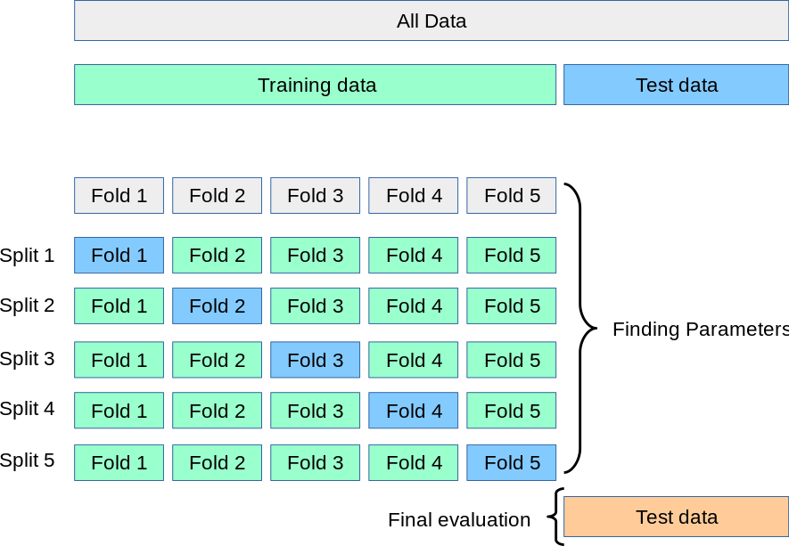
overfitting을 막기 위해서 데이터를 쪼갠 다름에 k개로 나누어 train데이터 안에서도 일부는 훈련, 일부는 테스트 데이터 셋으로 나뉜다.
repeated k-fold는 이러한 과정을 N번 반복하며, 과정마다 각기 다른 데이터 셋이 훈련 및 테스트된다.
macro average ROC curve란?
세 그룹 이상 범주형 데이터를 분류할때, ROC curve를 나타내는 방법을 말한다.
만약 A, B, C그룹이 있다면, A vs B + C로 분류의 정확도를 비교하여 평균 내는 방법이다.
Multiclass Receiver Operating Characteristic (ROC)
Multiclass Receiver Operating Characteristic (ROC)
This example describes the use of the Receiver Operating Characteristic (ROC) metric to evaluate the quality of multiclass classifiers. ROC curves typically feature true positive rate (TPR) on the ...
scikit-learn.org
먼저, 여러 분류기에서 macro average ROC-curve를 그려보자
import numpy as np
import pandas as pd
import matplotlib.pyplot as plt

from itertools import cycle
from sklearn.datasets import load_iris
from sklearn.model_selection import train_test_split, RepeatedKFold
from sklearn.linear_model import LogisticRegression
from sklearn.ensemble import RandomForestClassifier
from sklearn.neighbors import KNeighborsClassifier
from xgboost import XGBClassifier
from sklearn.svm import SVC
from sklearn.neural_network import MLPClassifier
from sklearn.metrics import RocCurveDisplay, roc_curve, auc
from sklearn.preprocessing import LabelBinarizer, LabelEncoder, label_binarize

import xgboost as xgb  # Import XGBoost
from sklearn.datasets import load_iris
import random
여러 분류기 정의
classifiers = {
    'XGBoost': xgb.XGBClassifier(),  # Add XGBoost classifier
    'Neural Network': MLPClassifier(max_iter=1000),
    'Random Forest': RandomForestClassifier(),
    'Logistic Regression':  LogisticRegression(max_iter=1000),
    'Support Vector Machine': SVC(probability=True),
    'k-Nearest Neighbors': KNeighborsClassifier(),
}
# Example for logistic regression
classifier = LogisticRegression(max_iter=1000)
# Example for neural network (MLP)
classifier = MLPClassifier(max_iter=1000)
iris dataset불러오기
iris = load_iris()
target_names = iris.target_names
X, y = iris.data, iris.target
y = iris.target_names[y]

random_state = np.random.RandomState(0)
n_samples, n_features = X.shape
n_classes = len(np.unique(y))


# 데이터 셋 나누기
X_train, X_test, y_train, y_test = train_test_split(X, y, test_size=0.5, stratify=y, random_state=42)

# 클래스 레이블을 숫자로 인코딩
label_encoder = LabelEncoder()
y_train = label_encoder.fit_transform(y_train)
y_test = label_encoder.transform(y_test)
y_test여기서는 데이터 셋을 50대 50으로 나누었는데 보통 7:3이나 8:2가 일반적이다.
그러나 예제 스크립트에 써있는 형식으로 계산해 보겠다.
from itertools import cycle

fig, ax = plt.subplots(figsize=(6, 6))

# Initialize variables for macro-average ROC curve


for clf_name, classifier in classifiers.items():
    # Initialize variables to store ROC curve values
    fpr = {}
    tpr = {}
    roc_auc = {}

    fpr_grid = np.linspace(0.0, 1.0, 1000)
    mean_tpr = np.zeros_like(fpr_grid)

    # Fit the classifier and predict probabilities
    y_score = classifier.fit(X_train, y_train).predict_proba(X_test)

    label_binarizer = LabelBinarizer().fit(y_train)
    y_onehot_test = label_binarizer.transform(y_test)

    for i in range(len(target_names)):
        fpr[i], tpr[i], _ = roc_curve(y_onehot_test[:, i], y_score[:, i])
        roc_auc[i] = auc(fpr[i], tpr[i])

    # Interpolate all ROC curves at these points for macro-average
    for i in range(len(target_names)):
        mean_tpr += np.interp(fpr_grid, fpr[i], tpr[i])

    mean_tpr /= len(target_names)

    fpr[clf_name] = fpr_grid
    tpr[clf_name] = mean_tpr
    roc_auc[clf_name] = auc(fpr[clf_name], tpr[clf_name])

    print(f"Macro-averaged One-vs-Rest ROC AUC score for {clf_name}:\n{roc_auc[clf_name]:.2f}")

    # Plot the ROC curve for the classifier
    plt.plot(
        fpr[clf_name],
        tpr[clf_name],
        lw=2,
        label=f"{clf_name} (AUC = {roc_auc[clf_name]:.3f})"
    )

# Plot the chance-level line
plt.plot([0, 1], [0, 1], color="gray", lw=2, linestyle="--")

# Set plot properties
plt.axis("square")
plt.xlabel("False Positive Rate")
plt.ylabel("True Positive Rate")
plt.title("Macro-averaged One-vs-Rest ROC AUC score")
plt.legend(loc="lower right")
plt.show()


# Macro-averaged One-vs-Rest ROC AUC score for XGBoost:0.99
# Macro-averaged One-vs-Rest ROC AUC score for Neural Network:0.41
# Macro-averaged One-vs-Rest ROC AUC score for Random Forest:0.89
# Macro-averaged One-vs-Rest ROC AUC score for Logistic Regression:0.74
# Macro-averaged One-vs-Rest ROC AUC score for Support Vector Machine:0.37
# Macro-averaged One-vs-Rest ROC AUC score for k-Nearest Neighbors:0.58
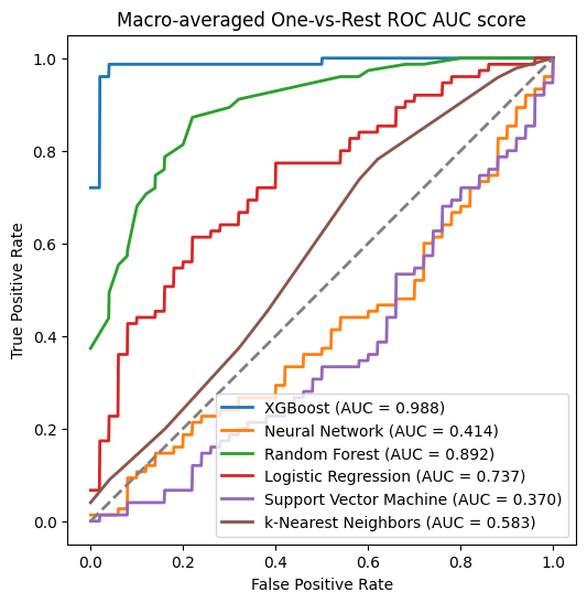
ROC curve의 0.0부분이 왜 잘렸는지는 의문이지만, 여러 분류기의 정확도가 계산되었다.
XGboost가 가장 훌륭한 정적을 보였으며, 그다음으로는 random forest, logstic regression이 뒤를 잇는다.
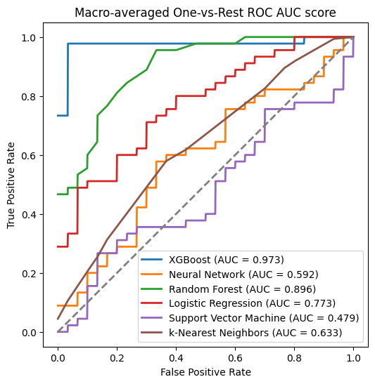
그러면 5 fold 3 repeated cross validation을 적용해 보자.
이때는 테스트 데이터 셋을 0.3, 훈련 데이터 셋을 0.7로 잡아보자
일단 아래는 cross validation을 사용하기 전, 데이터 셋을 7:3으로 잡은 결과이다
fig, ax = plt.subplots(figsize=(6, 6))
from itertools import cycle

random.seed(42)
np.random.seed(42)


# Initialize 5-fold 3-repeat cross-validation
n_splits = 5
n_repeats = 3
rkf = RepeatedKFold(n_splits=n_splits, n_repeats=n_repeats, random_state=42)

# Initialize variables for macro-average ROC curve
fpr_grid = np.linspace(0.0, 1.0, 1000)
mean_tpr = np.zeros_like(fpr_grid)


for clf_name, classifier in classifiers.items():
    # Initialize variables to store ROC curve values
    fpr = {}
    tpr = {}
    roc_auc = {}


    # Iterate over each fold in Repeated K-Fold
    for train_idx, test_idx in rkf.split(X_train):
        X_train_fold, X_test_fold = X_train[train_idx], X_train[test_idx]
        y_train_fold, y_test_fold = y_train[train_idx], y_train[test_idx]

        # Fit the classifier and predict probabilities for the fold
        random.seed(42)
        y_score = classifier.fit(X_train_fold, y_train_fold).predict_proba(X_test_fold)


        label_binarizer = LabelBinarizer().fit(y_train_fold)
        y_onehot_test = label_binarizer.transform(y_test_fold)


        for i in range(n_classes):
            fpr[i], tpr[i], _ = roc_curve(y_onehot_test[:, i], y_score[:, i])
            roc_auc[i] = auc(fpr[i], tpr[i])

        # Interpolate all ROC curves at these points for macro-average
        for i in range(n_classes):
            mean_tpr += np.interp(fpr_grid, fpr[i], tpr[i]) # linear interpolation


    # 교차 검증 값으로 단순히 나누어 주면 된다 ★★
    mean_tpr /= (n_splits * n_repeats * n_classes)

    fpr[clf_name] = fpr_grid
    tpr[clf_name] = mean_tpr
    #fpr["macro"] = np.insert(fpr["macro"], 0, 0)
    #tpr["macro"] = np.insert(tpr["macro"], 0, 0)
    roc_auc[clf_name] = auc(fpr[clf_name], tpr[clf_name])

    print(f"Macro-averaged One-vs-Rest ROC AUC score:\n{roc_auc[clf_name]:.3f}")

    # Plot the ROC curve for the classifier
    plt.plot(
        fpr[clf_name],
        tpr[clf_name],
        lw=2,
        label=f"{clf_name} (AUC = {roc_auc[clf_name]:.3f})"# ,
        # linestyle=":"
    )


    # Plot the chance-level line
plt.plot([0, 1], [0, 1], color="gray", lw=2, linestyle="--")

# Set plot properties
plt.axis("square")
plt.xlabel("False Positive Rate")
plt.ylabel("True Positive Rate")
plt.title("Macro-averaged One-vs-Rest ROC AUC score")
plt.legend(loc="lower right")
plt.show()
plt.tight_layout()

ax.plot([0,1,2], [10,20,3])
plt.show()

# Macro-averaged One-vs-Rest ROC AUC score: 0.991
# Macro-averaged One-vs-Rest ROC AUC score: 0.525
# Macro-averaged One-vs-Rest ROC AUC score: 0.945
# Macro-averaged One-vs-Rest ROC AUC score: 0.778
# Macro-averaged One-vs-Rest ROC AUC score: 0.658
# Macro-averaged One-vs-Rest ROC AUC score: 0.658
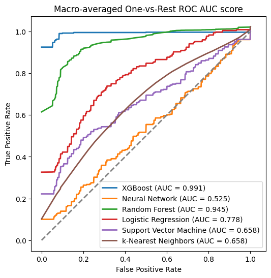
5 fold 3 repeated 교차 검증 후 정확도를 보니, random forest가 교차 검증 이전보다 정확도가 높아진 것을 볼 수 있다.
이를 토대로 안정적인 모델로 XGBoost과 randon forest를 사용하면 좋을 것이다.