
- 수정 : 2023.04.10.월
| 개요

미생물 샘플은 오염되는 경우가 매우 많다. 미생물은 눈에 보이지 않을뿐더러 공기 중에도 다수 존재하기 때문이다.
교수님께서 예전에 면봉으로 샘플링한 피부샘플이 대부분 오염된 걸로 판명되어서 샘플링 방법 체계를 다시 갖추셨다고 한다.
보통 Microbiome 하면 대변샘플을 가장 많이 연구하는데, 내가 분석하는 Skin 샘플은 오염도 쉽고 샘플링도 잘 안 되는 경우가 많다. 그래서 control sample과 비교하여 오염으로 판별된 서열을 제거해 주어야 한다.
이를 위한 프로그램으로는 R언어로 만들어진 decontam이 있다. (무려 dada2개발진이 만든 프로그램이다.) 이 프로그램의 튜토리얼을 소개하겠다.
- 튜토리얼 홈페이지 : https://benjjneb.github.io/decontam/vignettes/decontam_intro.html
| Decontam의 오염제거 방법 두 가지
- Frequency-based decontamination : 이 방법은 특정 OTU가 Negative control 샘플에서 매우 높은 빈도로 나타나면, 해당 OTU나 유전자가 True샘플이 아니라 공기 중의 오염된 균들이라고 가정한다. True 샘플에서 이러한 빈도가 높은 OTU를 제거하여 데이터 내의 오염을 감소시킨다.
- Prevalence-based decontamination : 이 방법은 여러 샘플에서 특정 OTU나 유전자가 나타나는 빈도를 분석하여, 해당 OTU나 유전자가 모든 샘플에서 균일하게 나타나지 않는 경우, 해당 OTU가 오염일 가능성이 높다고 가정한다. 이 방법은 이러한 균일하지 않은 분포를 가진 OTU나 유전자를 제거하여 데이터 내의 오염을 감소시킨다.
이 중에서는 1.Frequency-based decontamination 에 대해서 살펴볼 것이다.
| 1. Frequency-based decontamination
# 초기 세팅
library(phyloseq)
library(tidyverse)
#install.packages("decontam")
library(decontam)


# 패키지에 포함된 예제 데이타
ps <- readRDS(system.file("extdata", "MUClite.rds", package="decontam"))
# phyloseq-class experiment-level object
#  otu_table()   OTU Table:         [ 1951 taxa and 569 samples ]
#  sample_data() Sample Data:       [ 569 samples by 6 sample variables ]
#  tax_table()   Taxonomy Table:    [ 1951 taxa by 6 taxonomic ranks ]


head(sample_data(ps), 10)
tail(sample_data(ps), 10)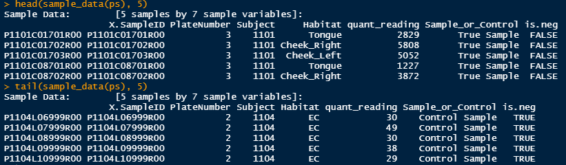
True sample이 우리가 분석하고자 하는 sample이며, Control Sample이 샘플 채취 환경에 공기 중에 노출한 sample이다.
우리는 공기 중에 있는 미생물이 샘플링에도 오염됐을 것이라 가정하여 control sample에 확인된 otu를 제거하려는 것이다.
# Inspect Library Sizes
df <- as.data.frame(sample_data(ps)) # Put sample_data into a ggplot-friendly data.frame
df$LibrarySize <- sample_sums(ps)
df <- df[order(df$LibrarySize),]
df$Index <- seq(nrow(df))
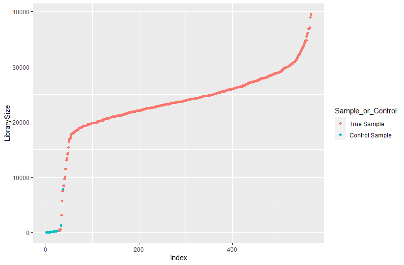
ggplot(data=df, aes(x=Index, y=LibrarySize, color=Sample_or_Control)) + geom_point()
LibrarySize란 각 sample의 read의 수의 하버를 나타낸다.
True Sample을 read수가 20000을 넘는 게 대부분인 반면에
Control Sample은 대다수가 5000 이하이다.
Control Sample은 공기 중에 미생물 혹은 sampling시 추출하려는 부분 외에 다른 곳에 닿았을 때 묻어난 미생물의 서열임으로 그 수가 많지 않은 것을 볼 수 있다.
우리가 decontam으로 할 것을 각 샘플이 겹치는 구간을 제거하는 것인데, 이때 우리는 얼마나 'frequency'방법으로 오염된 ASV를 구할 것이다. 이는 ASV 단위로 오염됐는지 아닌지를 판별한다는 뜻이다.
이 frequency방법에서 고려되는 변수는 quant_reading이다. 이 값은 PCR직후 각 샘플에서 측정된 DNA의 농도를 말한다. 만약 이 값이 존재하지 않는다면 아래 방법을 Prevalence 사용하는 것을 추천한다.
# Identify Contaminants - Frequency
contamdf.freq <- isContaminant(ps, method="frequency", conc="quant_reading")

head(contamdf.freq)
table(contamdf.freq$contaminant)
#   FALSE  TRUE
#    1893    58
which(contamdf.freq$contaminant)
#  [1]    3   30   53   80  152  175  176  193  196  197  206  230  238  243  265  272  273  286  298  307  309  330
# [23]  333  382  389  395  409  411  416  420  422  426  434  444  460  472  473  476  488  489  576  578  584  599
# [45] 607 608 632 643 667 717 734 736 812 813 853 1041 1069 1661결과를 보니 3번째로 sample에 풍부(!)하다고 나온 ASV가 Control Sample에서 발견되어 오염으로 판별되었다.
이때 3번째 서열이 진짜 오염인지 다시 한번 판별할 필요가 있다.
오염으로 판별된 ASV3와 정상 sample에서 발견된 ASV1을 비교해 보자.
plot_frequency(ps, taxa_names(ps)[c(1,3)], conc="quant_reading") +
  xlab("DNA Concentration (PicoGreen fluorescent intensity)")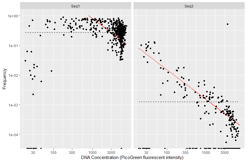
빨간 선이 오염됐다고 보는 model이다. seq3는 빨간 선과 비슷한 모양을 보인다.
그러므로 3번째로 풍부한 ASV이지만 오염되었으니 삭제해도 무방하다.
다른 오염된 ASV도 보자.
set.seed(100)
plot_frequency(ps, taxa_names(ps)[sample(which(contamdf.freq$contaminant),3)], conc="quant_reading") +
  xlab("DNA Concentration (PicoGreen fluorescent intensity)")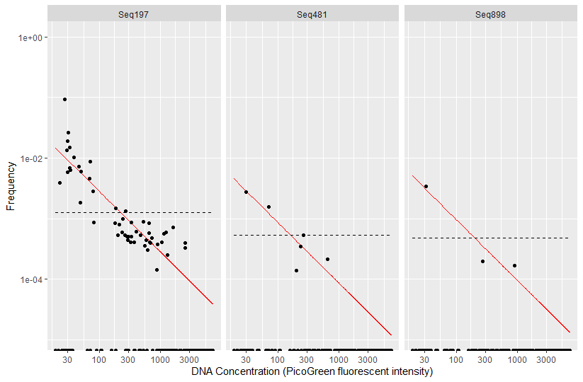
다 빨간 선과 비슷한 추세를 보임으로 오염된 ASV이다.
ps
# phyloseq-class experiment-level object
# otu_table()   OTU Table:         [ 1951 taxa and 569 samples ]
# sample_data() Sample Data:       [ 569 samples by 7 sample variables ]
# tax_table()   Taxonomy Table:    [ 1951 taxa by 6 taxonomic ranks ]

ps.noncontam <- prune_taxa(!contamdf.freq$contaminant, ps)
ps.noncontam
# phyloseq-class experiment-level object
# otu_table()   OTU Table:         [ 1893 taxa and 569 samples ]
# sample_data() Sample Data:       [ 569 samples by 7 sample variables ]
# tax_table() Taxonomy Table: [ 1893 taxa by 6 taxonomic ranks ]오염된 ASV를 제외하면 1893개의 ASV만 남게 된다.
df <- as.data.frame(sample_data(ps.noncontam)) # Put sample_data into a ggplot-friendly data.frame
df$LibrarySize <- sample_sums(ps.noncontam)
df <- df[order(df$LibrarySize),]
df$Index <- seq(nrow(df))
ggplot(data=df, aes(x=Index, y=LibrarySize, color=Sample_or_Control)) + geom_point()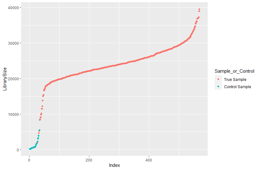
decontam과 비교해 보면 control sample과 겹치던 부분이 상당수 제거된 것을 볼 수 있다.
다음 편에는 decontam 모델 중 Prevalence를 이용한 오염판별을 보겠다.
| 2. Prevalence-based decontamination
일단 기존 샘플에서 Prevalence를 이용해서 오염서열을 판별해 보자. 이는 taxa의 abundance를 고려하는 것이 아니라, Negative Control에서 존재하는 패턴을 기준으로 구분한다(출처). 기존의 default threshold값은 0.1이지만, Prevalence에서는 기준점을 0.5로 잡는다. 값을 여유롭게 잡아야 positive 샘플에서 더 많은 서열을 감지할 수 있다.
contamdf.prev05 <- isContaminant(ps, method="prevalence", neg="is.neg", threshold=0.5)
table(contamdf.prev05$contaminant)
# FALSE  TRUE
# 1809   142
제거된 ASV의 수를 관찰해 보자.
ps.noncontam.prev <- prune_taxa(!contamdf.prev05$contaminant, ps)
ps.noncontam.prev
# phyloseq-class experiment-level object
# otu_table()   OTU Table:         [ 1809 taxa and 569 samples ]
# sample_data() Sample Data:       [ 569 samples by 7 sample variables ]
# tax_table() Taxonomy Table: [ 1809 taxa by 6 taxonomic ranks ]오염된 ASV를 제외하면 1809개의 ASV만 남게 된다.
오염으로 판별된 서열과 True판별된 서열의 Prevalance를 살펴보자
# Make phyloseq object of presence-absence in negative controls and true samples
ps.pa <- transform_sample_counts(ps, function(abund) 1*(abund>0))
ps.pa.neg <- prune_samples(sample_data(ps.pa)$Sample_or_Control == "Control Sample", ps.pa)
ps.pa.pos <- prune_samples(sample_data(ps.pa)$Sample_or_Control == "True Sample", ps.pa)
# Make data.frame of prevalence in positive and negative samples
df.pa <- data.frame(pa.pos=taxa_sums(ps.pa.pos), pa.neg=taxa_sums(ps.pa.neg),
                    contaminant=contamdf.prev$contaminant)
ggplot(data=df.pa, aes(x=pa.neg, y=pa.pos, color=contaminant)) + geom_point() +
  xlab("Prevalence (Negative Controls)") + ylab("Prevalence (True Samples)")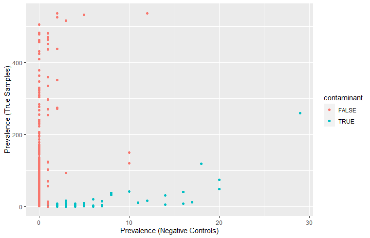
Negative Control에서 Prevalance가 높은 서열이 오염(True)으로 인식된 것을 볼 수 있다.
| Prevalence vs Frequency (feat. chatGPT)
- Prevalence-based decontamination은 일반적으로 더 보수적인 접근 방식이다. 이 방법은 상대적으로 드문 오염 균주를 감지할 수 있어 적은 양의 오염 데이터를 식별할 수 있다는 장점이 있다. 그러나 이 방법은 덜 민감하며, 정확성이 낮을 수 있다는 단점이 있다. 또한 드문 오염 균주를 식별하면서 실제로 유익한 미생물 균주를 오염으로 잘못 식별할 수 있다.
- 반면, Frequency-based decontamination은 오염 균주를 더 잘 식별할 수 있지만, 그만큼 더 많은 유익한 미생물 균주를 잘못 제거할 수도 있다. 이 방법은 민감한 접근 방식이므로 적은 양의 오염 데이터를 식별하는 데 유용하다. 또한, 이 방법은 더 높은 정확도를 가지며, 특히 고용량 데이터셋에서 유용하다.
- 따라서, Prevalence-based decontamination은 드문 오염 균주를 식별하면서 잘못된 유익한 미생물 균주의 감소를 가져올 수 있지만, Frequency-based decontamination은 보다 높은 정확도를 가지며 민감한 접근 방식으로 더 많은 오염 데이터를 식별할 수 있다는 장점이 있다.
- 선택해야 하는 방법은 분석의 목적과 데이터셋의 크기와 같은 여러 요인에 따라 다를 수 있다.
- 피부마이크로바이옴 데이터의 경우, 오염이 발생하기 쉽고 read가 적어 오염의 영향이 크다. Prevalence 방법은 해당 OTU가 여러 샘플에서 나타나는 정도를 고려하기 때문에, 여러 샘플에서 검출되는 OTU를 더 잘 잡아낸다. 그러므로 적은 수의 시퀀싱 read에서도 오염을 잘 식별할 수 있다. 그러나 frequency 방법의 경우, 특정 OTU가 검출되는 비율에 따라 오염을 식별한다. 이 경우에서는 read수가 적을수록 잘 감지하지 못할 수도 있다.